R for Sound Analysis Tutorial

library(ggplot2)
library(umap)
library(seewave)
library(tuneR)
library(phonTools)
library(signal)
library(warbleR)

# Part I.  Read in sound files and spectrograms ---------------------------

# We can easily read in the sound file using the following line of code
LongSoundFile <- tuneR::readWave('S11_20180319_060002.wav')

# Now we can check the structure of the resulting .wav file
LongSoundFile@left[1:5] # This returns the values of the waveform
## [1] -1038  -722   171  -148  -504
LongSoundFile@samp.rate # This is the sampling rate
## [1] 16000

# We can also read in the selection table made in Raven using the following code
SelectionTableName <- 'VirtualClusteringExample_S11_20180319_060002.Table.1.selections.txt' 

SoundscapeTable <- read.delim(SelectionTableName,
           stringsAsFactors = F)

# Now we want to check the structure of the table
# str(SoundscapeTable)
# head(SoundscapeTable)

# This selection table has annotations of different call types
table(SoundscapeTable$Call.type)
## 
##         argus         bird1         bird2 female.gibbon       insect1 
##             7             5             5             5             5

# We can use the Raven selection table to isolate these particular sounds
ListofWavs <- lapply(1:nrow(SoundscapeTable), function(x) cutw(LongSoundFile, from=SoundscapeTable$Begin.Time..s.[x],
                                                 to=SoundscapeTable$End.Time..s.[x], output='Wave'))

# We now have a list of .wav files that were created from our Raven selection table. If we want we can save them to a local directory
dir.create('SoundFiles') # This line creates a folder in your working directory

# This loop will write the shorter sound files to the directory indicated above
for(x in 1:length(ListofWavs)){
  writeWave(ListofWavs[[x]], 
            filename= paste('SoundFiles','/',SoundscapeTable$Call.type[x],
                            '_', x, '.wav',sep=''))
}

# Now we can make a spectrogram. First lets read in the .wav file
FemaleGibbonFile <- readWave("SoundFiles/female.gibbon_2.wav")

# There are many different packages that you can use to create spectrograms
# This is a spectrogram from 'seewave'
seewave::spectro(FemaleGibbonFile,flim=c(0,3))

# Lets check out spectrograms of all the signals
GreatArgusFile <- readWave("SoundFiles/female.gibbon_2.wav")
Bird1File  <- readWave("SoundFiles/bird1_9.wav")
Bird2File <- readWave("SoundFiles/bird2_20.wav")
Insect1File <- readWave("SoundFiles/insect1_24.wav")

seewave::spectro(FemaleGibbonFile,flim=c(0,3))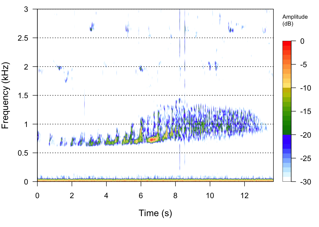

seewave::spectro(Bird1File,flim=c(0,3))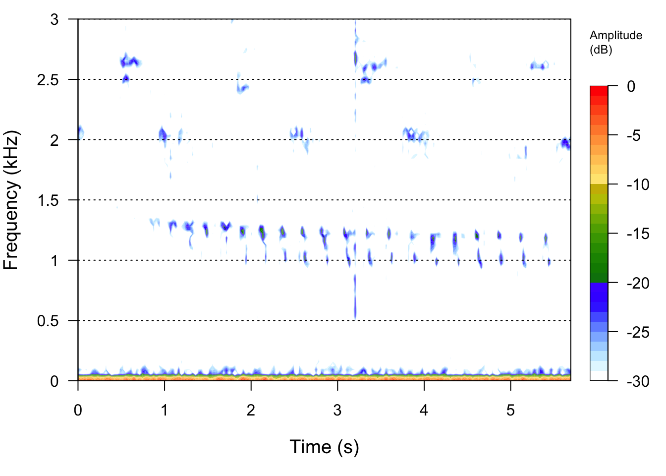

seewave::spectro(Bird2File,flim=c(0,3))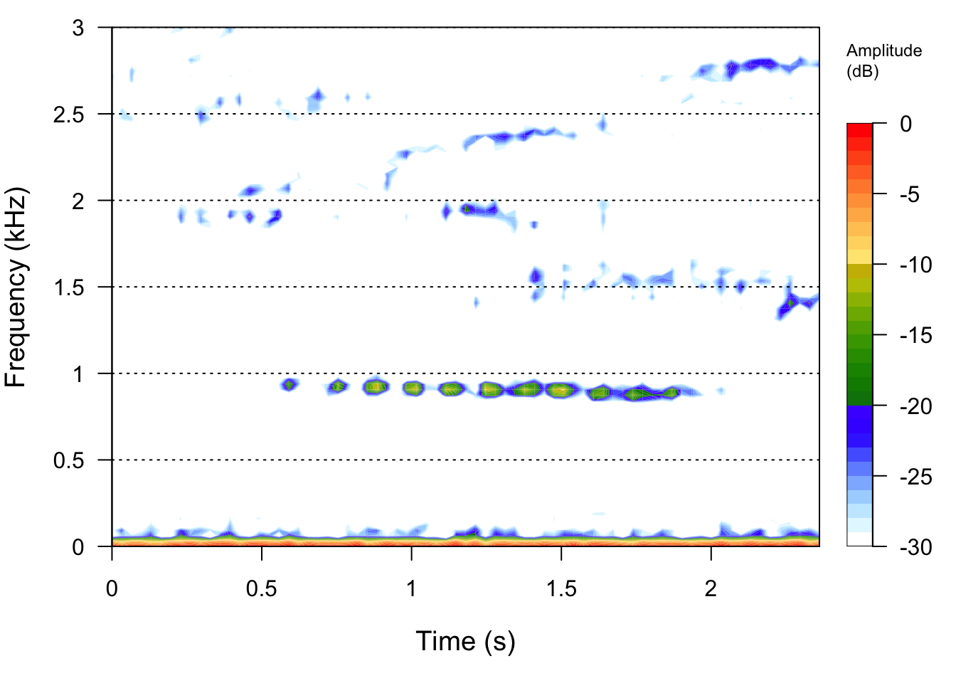

seewave::spectro(Insect1File,flim=c(3,6))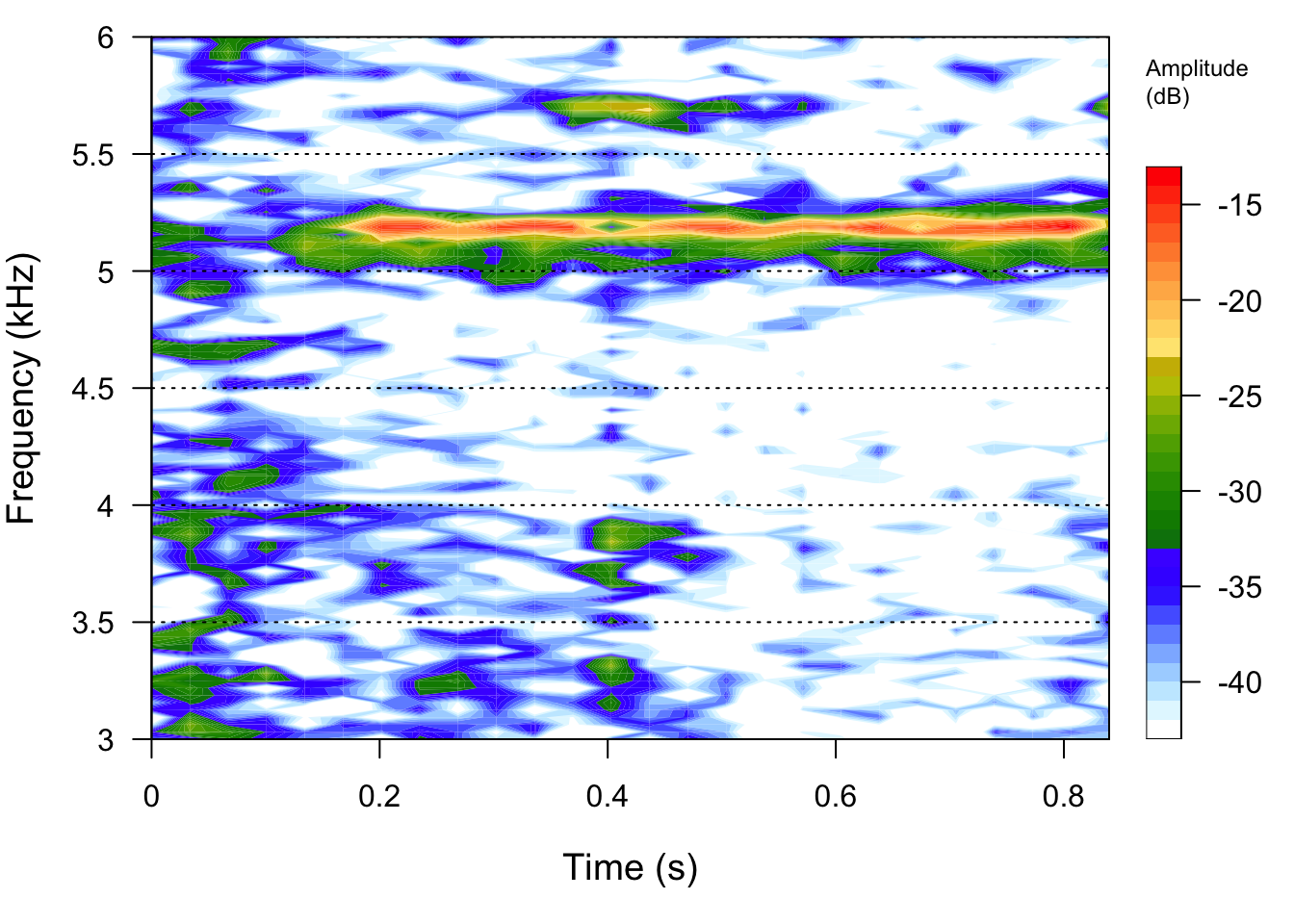

# Part 2.  Unsupervised classification ------------------------------------

# Our Raven selection table also has some potentially useful features for distinguishing between call types
#str(SoundscapeTable)

# First let's try a more traditional unsupervised approach- PCA
BorneoCallTypes.pca <- 
 princomp(SoundscapeTable[,c(8:11)])

plot.for.BorneoCallTypes <-
  cbind.data.frame(BorneoCallTypes.pca$scores [,1:2],
                   SoundscapeTable$Call.type)

colnames(plot.for.BorneoCallTypes) <-
  c("Dim.1", "Dim.2", "Call.type")

my_plot_BorneoCallTypes.pca <-
  ggplot(data = plot.for.BorneoCallTypes, aes(
    x = Dim.1,
    y = Dim.2,
    colour = Call.type
  )) +
  geom_point(size = 3) +
  scale_color_manual(values = matlab::jet.colors (length(unique(plot.for.BorneoCallTypes$Call.type)))) +
  theme_bw() + ggtitle('Borneo call types') + xlab('pca: Dim 1')+ylab('pca: Dim 2')#+ theme(legend.position = "none")

my_plot_BorneoCallTypes.pca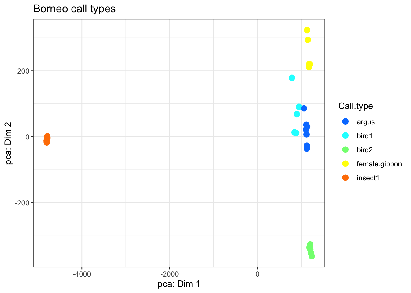

# Now we can use Uniform Manifold Approximation and Projection for Dimension Reduction

BorneoCallTypes.umap <- 
  umap::umap(SoundscapeTable[,c(8:11)],labels=as.factor(SoundscapeTable$Call.type),
             controlscale=TRUE,scale=3)

plot.for.BorneoCallTypes <-
  cbind.data.frame(BorneoCallTypes.umap$layout[,1:2],
                   SoundscapeTable$Call.type)

colnames(plot.for.BorneoCallTypes) <-
  c("Dim.1", "Dim.2", "Call.type")

my_plot_BorneoCallTypes <-
  ggplot(data = plot.for.BorneoCallTypes, aes(
    x = Dim.1,
    y = Dim.2,
    colour = Call.type
  )) +
  geom_point(size = 3) +
  scale_color_manual(values = matlab::jet.colors (length(unique(plot.for.BorneoCallTypes$Call.type)))) +
  theme_bw() + ggtitle('Borneo call types') + xlab('UMAP: Dim 1')+ylab('UMAP: Dim 2')#+ theme(legend.position = "none")

my_plot_BorneoCallTypes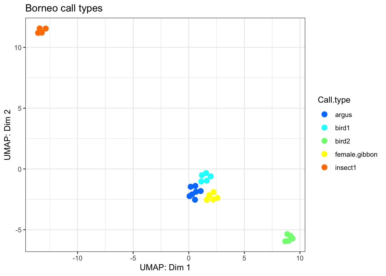

# Part 4.  Supervised classification --------------------------------------
LDAdata <- SoundscapeTable[,-c(1:5)]

lda.output <- MASS::lda(
  Call.type  ~ .,
  data=LDAdata,
  center = TRUE,
  scale. = TRUE,
  CV = T
)

# Assess how well the leave one out cross validation did
ct <-
  table(grouping = LDAdata$Call.type, lda.output$class)

# Check structure of the table
ct
##                
## grouping        argus bird1 bird2 female.gibbon insect1
##   argus             7     0     0             0       0
##   bird1             0     5     0             0       0
##   bird2             0     0     5             0       0
##   female.gibbon     0     0     0             5       0
##   insect1           0     0     0             0       5

# Calculate total percent correct
percent <- sum(diag(prop.table(ct)))*100
percent
## [1] 100


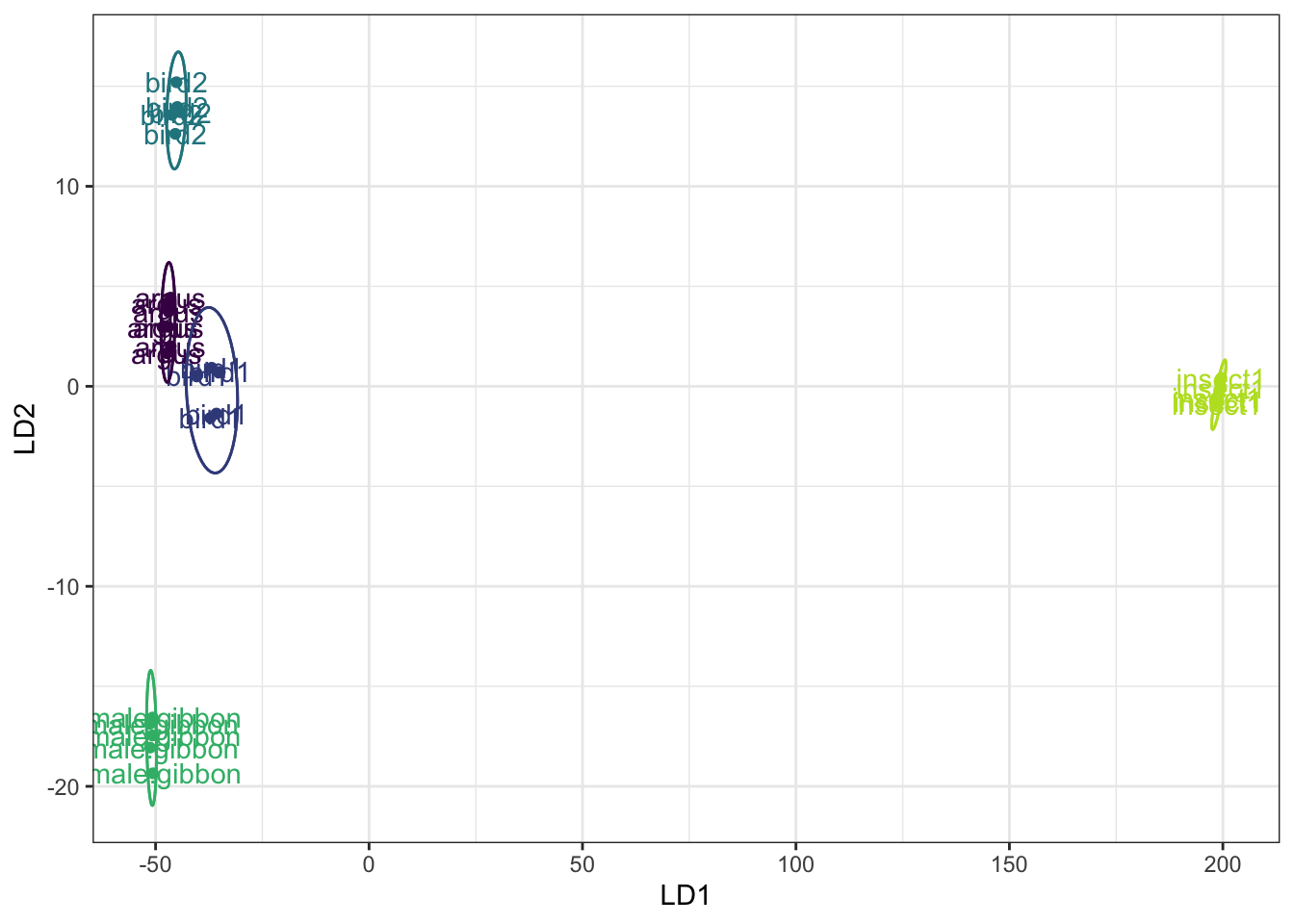
# Now we can create a biplot based on the LDA
fit.lda <- MASS::lda(Call.type ~ ., LDAdata)
class.lda.values <- predict(fit.lda)

# Combine the results into a new dataframe
newdata <- data.frame(class = LDAdata$Call.type, lda = class.lda.values$x)

# Code to create the plot
lda.plot <- ggplot(newdata, aes(lda.LD1, lda.LD2, colour = class)) + 
  geom_point() + geom_text(aes(label = class)) + stat_ellipse() + xlab("LD1") + ylab("LD2") + 
  stat_ellipse(aes(lda.LD1, lda.LD2)) + theme(legend.position = "") + theme(axis.text.x = element_text(size = 20)) + 
  theme(axis.text.y = element_text(size = 20)) + theme(axis.title.x = element_text(size = 20)) + 
  theme(axis.title.y = element_text(size = 20)) + viridis::scale_color_viridis(discrete = T, end = 0.9) + 
  theme(panel.grid.major = element_blank(), panel.grid.minor = element_blank(), axis.line = element_blank()) + 
  guides(colour = FALSE) +theme_bw()

lda.plot